Session 8: Plotting Graphs with Matplotlib
Date: 25-04-2026 4:00 pm to 6:00 pm
Agenda
- Review of previous sessions
- Answers to queries
- Introduction to Matplotlib
- Python Modules
Introduction to Matplotlib
The Matplotlib homepage describes Matplotlib as:
From Matplotlib home page
Matplotlib is a comprehensive library for creating static, animated, and interactive visualizations in Python. Matplotlib makes easy things easy and hard things possible.
It relies on NumPy for the ndarray data structure to store data and provides the functions to plot a wide variety of graphs. Being one of the earliest data visualization library for Python, it is very popular and widely used. There are several more recent plotting libraries for Python, but Matplotlib remains relevant and popular.
Matplotlib will appear familiar to Matlab users as its traditional approach to generating plots parallel those of Matlab. However, the current style of using Matplotlib uses the object oriented approach that is a little different. While Matplotlib can generate several types of graphs, this introduction will restrict itself primarily to plotting line graphs and perhaps a few other realted graphs.
Installing Matplotlib
Matplotlib depends on NumPy and if NumPy is not already installed, it will be installed automatically.
Once installed, open the Python REPL, import matplotlib and check its version to confirm it was installed correctly:
The typical workflow consists of:
- Import the
matplotlib.pyplotsubpackage aspltonce in each script or program which usesmatplotlib. - Prepare or create the data to be plotted.
- Initialize a
plt.subplots()and store the values of figure and axis returned by it. - Use the axis to execute one or more
plot()orset()methods. - Display the plot with the
plt.show()function call.
Plot graphs of sin and cos
The example below plots a graph of sin and cos for values from \(0\) to say \(2 \pi\):
>>> import matplotlib.pyplot as plt
>>> import numpy as np
>>> x = np.linspace(0, 2 * np.pi, 129)
>>> y1 = np.sin(x)
>>> y2 = np.cos(x)
>>> fig, ax = plt.subplots()
>>> ax.plot(x, y1)
>>> ax.plot(x, y2)
>>> ax.grid()
>>> ax.set_xlabel("x")
>>> ax.set_ylabel("y")
>>> ax.set_title(r"Graphs of $\sin$ and $\cos$")
>>> plt.show()
This will pop up a window with the plot, and the menu at the bottom lets you save the image to the filesystem.
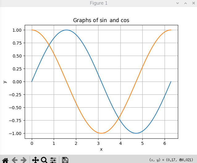
Note
- The colours of the lines are chosen automatically, but it can be specified if needed.
- Other settings allow the programmer to choose the thickness of the lines, the style of the lines, markers at the data points, limits for the axes, intervals for the tic marks etc.
- The labels can contain \(\LaTeX\) markup to generate greek letters, super and sub-scripts etc.
- It is possible to place a legend at one of the corners (or other specific location).
- It is possible to annotate the plots.
Multiple sub-plots
import matplotlib.pyplot as plt
import numpy as np


def f(t):
    return np.exp(-t) * np.cos(2*np.pi*t)

t1 = np.arange(0.0, 5.0, 0.1)
t2 = np.arange(0.0, 5.0, 0.02)

fig, ax = plt.subplots(nrows=2, ncols=1)
ax[0].plot(t1, f(t1), 'bo', t2, f(t2), 'k')

ax[1].plot(t2, np.cos(2*np.pi*t2), 'r--')
plt.show()
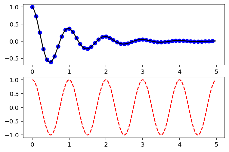
Note
- The arguments
nrows=2andncols=1toplt.subplots()specify the number of rows and columns to split the figure into. - The list
axtherefore has two elements (2 rows and 1 column) and each is indexed asax[0]andax[1]. - The plot output is directed to the specific subplot based on the chosen
ax.
See the Matplotlib Tutorials page for more examples.
The stress-strain relation for concrete is given by the expression:
Define a function to calculate the stress (\(f_c\)) for given value of strain (\(\epsilon_c\)) and plot a graph of strain vs stress.
Note
- The function
fc(ec, fck, ecy, ecu)calculates the stressfcfor one given value ofec - The
v_fc = np.vectorize(fc)converts the functionfc()to vector formv_fc()so that the functionfc()can be applied to each element of anndarraywithout writing aforloop.
Create the array ec to store the data points at which \(f_c\) is to be calculated. Since there are two distinct portins of the graph, namely \(0 \leq \epsilon_c < \epsilon_{cy}\) and \(\epsilon_{cy} \leq \epsilon_c \leq \epsilon_{cu}\), generate two 1D arrays and concatenate them.
np.linspace(0, ecy, 51)generates51equally spaced points from0toecy.np.linspace(ecy, ecu, 5)generates5equally spaced points fromecytoecu.np.concat((np.linspace(0, ecy, 51), np.linspace(ecy, ecu, 5)))concatenates the two arrays, resulting in a length of56elements.
The output should be
The plot can be generated as usual:
- The \(LaTeX\) markup for \(\epsilon_c\) is
$epsilon_c$and for \(f_c\) is$f_c$.
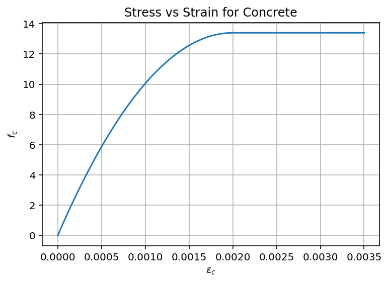
Key technique learnt
Converting a scalar function to vector form. Note that atleast one of the arguments to the vectorized function must be an array.
Understanding Modules and Packages
In the world of software, a module is a distinct part of a system that performs a specific function and works together with other parts. In Python, we use modules and packages to organize our code, making it easier to read, test, and reuse.
What is a Module?
While a single function is "modular," in Python, the term module specifically refers to a file containing Python code (ending in .py).
A module usually contains a collection of related functions, variables, or classes that serve a common purpose. By grouping related code into a module, you simplify complex tasks and keep your main program clean.
What is a Package?
The next level of organization is the package. A package is simply a collection of interrelated modules grouped together in a directory (folder). Think of a module as a single file and a package as a folder containing many of those files.
Where do Modules and Packages come from?
There are three main sources for the tools you will use in your programs:
-
The Python Standard Library (Built-in)
Python comes "batteries included." Many modules and packages are automatically installed when you install Python. These are known as the Standard Library.- Examples: The
mathmodule for calculations or thecollectionspackage for advanced data types. - Access: Since they are already on your system, you can use them immediately.
- Examples: The
-
External Packages (Third-Party)
These are created by the global Python community and hosted on services like PyPI. You must install these before you can use them (usually via a tool likepip).- Examples:
numpyfor scientific computing ormatplotlibfor creating graphs.
- Examples:
-
Your Own Modules (Custom)
As your programs grow, you should collect your own functions and constants into.pyfiles. This allows you to:- Stay Organized: Keep your main script short and focused.
- Increase Reusability: Use the same functions in different projects without rewriting them.
- Improve Testing: Test individual parts of your code independently.
How to Use Them
Regardless of where the module or package comes from, you bring it into your current program using the import keyword. This tells Python to load that specific code so you can use its features.
Understanding Namespaces
As you start using more modules and packages, you might worry: "What happens if I name a variable data, but a module I imported also has a variable named data?"
Python solves this problem using Namespaces.
What is a Namespace?
A namespace is essentially a naming system to ensure that all the names in your program (like variables, functions, and modules) stay organized and don't clash with each other.
Think of a namespace like a surname (last name):
- In a classroom, there might be two students named Rajesh. This is confusing.
- However, if one is Rajesh Patil and the other is Rajesh Kulkarni, there is no confusion.
- The surnames "Patil" and "Kulkarni" act like namespaces to keep the names distinct.
Why Namespaces Matter
In Python, namespaces allow you to use the same name for different things, as long as they live in different "folders." For example:
- The Global Namespace: This contains names defined in your main program.
- The Module Namespace: This contains names defined inside a specific module (like
mathorrandom). - The Local Namespace: This contains names defined inside a specific function.
A Real-World Example
If you import the math module, it has its own namespace. This is why you often see code like this:
import math

# This 'pi' belongs to the math namespace
print(math.pi)

# You can still create your own 'pi' in your program's namespace
pi = 3
print(pi)
By using math.pi, you are telling Python: "I want the pi that belongs to the math namespace, not the one I created myself." This keeps your code safe and organized!
Our first module - A module to operate on vectors
Let us create our own module to perform the following operations related to vectors:
- Create a vector as a one dimensioned list with three components.
- Add two vectors or subtract one from the other.
- Obtain the dot product of two vectors.
- Obtain the cross product of two vectors.
- Obtain magnitude, and
- Unit vector along the given vector.
Theory
Given two vectors \(A = A_x \, i + A_y \, j + A_z \, k\) and \(B = B_x \, i + B_y \, j + B_z \, k\), where \(i, j, k\) are unit vectors along the \(x, y, z\) axes respectively, the different operations are given below:
1. Addition or Subtraction: Result of addition or subtraction is a vector and is given by:
2. Dot Product: Dot product results in a scalar and is given by:
where \(\theta\) is the angle between \(A\) and \(B\). Applications of the dot product include determining the projection of one vector in the direction of another vector (\(A \cdot \hat{B} = |A| \cdot 1 \cdot \cos \theta = |A| \cos \theta\)) and determining the angle between two given vectors \(\left( \theta = \cos^{-1} \left( \frac{A \cdot B}{|A| |B|} \right) \right)\).
3. Cross Product: Cross product is a vector and is given by:
where \(\theta\) is the angle between \(A\) and \(B\) and \(\hat{n}\) is a unit vector normal to the plane of \(A\) and \(B\), positive as per the right hand rule. Magnitude of the cross product is the are of the parallelogram formed by the two vwctors. If the cross product is zer, either one or both vectors have zero magnitude or they are parallel, that is, \(\theta = 0^{\circ}\) or \(\theta = 180^{\circ}\).
4. Magnitude: Magnitude is a scalar given by:
5. Unit Vector: Unit vector along a given vector has the same direction as the given vector but has a unit magnitude. It is given by:
Python module
Open Python REPL and do the following:
Alternately, create a file namedmain.py or any name of your choice in a code editor such as VS Code and type the following:
| main.py | |
|---|---|
Tip
To not execute the lines of code meant to test the functions in this file when this file is imported as a module, put these lines in a conditional block if __name__ == "__main__".
Now, if you run the main.py file, it will produce no output. This is because:
- Import Logic: When a file is imported, Python executes all code in that file once.
- Unconditional Execution: Any code not inside the if name == "main": block runs automatically upon import.
- Conditional Execution: Python sets an internal variable named name for every file.
- When the file is executed directly, name is set to "main". The condition is met, and the test code runs.
- When the file is imported, name is set to the module name (e.g., "vector"). The condition is not met, and the test code is skipped.
You can verify this by adding a line print(__name__) above the conditional block:
| vector.py | |
|---|---|
If you execute vector.py directly, you will see main. If you execute main.py, you will see vector, and the test results will be hidden.
To use the module functions in main.py, use the module name as a prefix:
| main.py | |
|---|---|
main.py produces the same output as the test code in vector.py.
Creating Packages
While a module is a single .py file, a package is a collection of modules placed within a directory. In regular packages, the directory contains a special file named __init__.py. This file is often empty; however, if it contains code, that code is executed once when the package is first imported. Since Python 3.3, directories without an __init__.py are also recognized as namespace packages. The name of the directory defines the name of the package. Any .py files in this directory are treated as modules, and sub-directories are treated as sub-packages.
We will look at creating packages at a later point of time.